How To Freeze Cells in Excel For Specific Rows and Columns

You can freeze specific rows and columns in Excel by using the Freeze Panes feature. This function keeps selected rows or columns visible while you scroll through your worksheet. When you know how to freeze cells in excel, you make it easier to read large datasets and compare data points without losing track of headers.

Freezing rows and columns is especially useful in several business scenarios:

FineReport also supports advanced data management by integrating with Excel and offering powerful reporting features for business users.

How to Freeze Cells in Excel

Freezing cells in Excel helps you keep important information visible as you scroll through large datasets. When you learn how to freeze cells in excel, you can always see headers or key identifiers, which makes data analysis and navigation much easier. This section will guide you through freezing rows, columns, or both, and provide practical tips for avoiding common mistakes.

Freeze rows

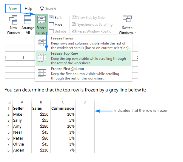
You often need to keep the top row or several rows visible while scrolling down your worksheet. This is especially useful for keeping column headers in view.

To freeze the top row:

1. Open your Excel worksheet.
2. Go to the View tab on the ribbon.
3. In the Window group, click Freeze Panes.
4. Select Freeze Top Row.

The top row will now stay visible as you scroll down. This method works in Excel 2016, 2019, and Microsoft 365.

To freeze multiple rows:

1. Select the cell in the first column, just below the last row you want to freeze. For example, to freeze the first three rows, select cell A4.
2. Go to the View tab.
3. Click Freeze Panes.
4. Choose Freeze Panes from the dropdown menu.

Now, all rows above your selected cell remain visible as you scroll.

Tip: Always select the cell directly below the last row you want to keep visible. If you select the wrong cell, you might not freeze the intended rows.

Freezing rows is a key part of how to freeze cells in excel, especially when working with large tables.

Freeze columns

Sometimes, you need to keep one or more columns visible while scrolling horizontally. This is helpful when your data has important row labels or identifiers.

To freeze the first column:

1. Go to the View tab.
2. Click Freeze Panes.
3. Select Freeze First Column.

The first column will now stay visible as you scroll right.

To freeze multiple columns:

1. Select the cell just to the right of the last column you want to freeze. For example, to freeze columns A and B, select cell C1.
2. Go to the View tab.
3. Click Freeze Panes.
4. Choose Freeze Panes from the dropdown.

This method keeps all columns to the left of your selected cell visible.

Note: If the Freeze Panes option is grayed out, check these common issues:

• Make sure you are in 'Normal' view. Go to the View tab and select 'Normal' in the Workbook Views section.
• Unprotect the worksheet if it is protected. Go to the Review tab and select 'Unprotect Sheet'.
• Unfreeze any existing panes before trying again.
• Check for hidden rows or columns, as these can interfere with freezing.
• If problems persist, try repairing the Excel file.

Freezing columns is another important aspect of how to freeze cells in excel, especially for wide datasets.

Freeze rows and columns

You may need to freeze both rows and columns at the same time. This is common when you want to keep both headers and row labels visible.

To freeze both rows and columns:

1. Make sure no panes are already frozen. Go to the View tab and select Unfreeze Panes if needed.
2. Select the cell that is immediately below the last row and immediately to the right of the last column you want to freeze. For example, to freeze the first two rows and the first two columns, select cell C3.
3. Go to the View tab.
4. Click Freeze Panes.
5. Choose Freeze Panes from the dropdown.

Everything above and to the left of your selected cell will remain visible as you scroll.

Tip: Selecting the correct cell is crucial. If you select the wrong cell, Excel may not freeze the intended rows and columns. Always double-check your selection before applying Freeze Panes.

Best Practice: Use Freeze Panes to keep headers visible in large datasets. This helps you avoid confusion and improves workflow efficiency. Data analysts often freeze both rows and columns to maintain visibility of key data points.

If you encounter issues where the Freeze Panes command does not work, check for these common problems:

• The worksheet is protected.
• You are not in 'Normal' view.
• There are hidden rows or columns.
• The Excel file may be corrupted.
• You are in cell editing mode.

Switch to 'Normal' view, unprotect the sheet, unhide any hidden rows or columns, and try again. Updating Excel to the latest version can also resolve some issues.

Learning how to freeze cells in excel gives you better control over your data. You can keep important information visible, reduce errors, and make your workflow more efficient. Whether you need to freeze rows, columns, or both, these steps will help you manage your spreadsheets with confidence.

Unfreeze Panes As Oppose To How to Freeze Cells in Excel

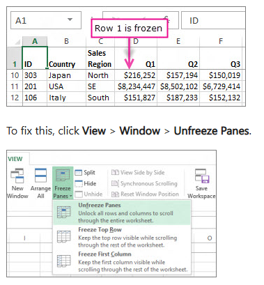
When you no longer need to keep certain rows or columns visible, you can easily unfreeze them in Excel. This restores your worksheet to its default scrolling behavior, letting you view all data without any locked sections.

Remove frozen rows and columns

You can unfreeze panes in just a few steps. The process works the same way in most versions of Excel, so you do not need to worry about which version you use.

Follow these steps to unfreeze panes:

1. Open your Excel worksheet where you have frozen rows or columns.
2. Go to the View tab on the ribbon.
3. In the Window group, select Unfreeze Panes.
4. If you prefer using shortcuts, on Windows you can press Alt + W + F + U.
5. Scroll through your worksheet to confirm that all previously frozen rows and columns are now unlocked.

You will find that these steps remain consistent across different versions of Excel. However, if you use Excel for Mac, you may not have a direct keyboard shortcut for unfreezing panes. In that case, use the menu options instead.

Tip: Unfreezing panes does not affect your data or formatting. It only changes how you view your worksheet.

Sometimes, you may encounter issues when trying to unfreeze panes. Use the table below to troubleshoot common problems:

If you want to remove frozen rows and columns from multiple worksheets at once, you can use advanced methods. For example, you can open the Visual Basic for Applications (VBA) editor, insert a module, and run a macro to unfreeze panes across all worksheets. Some third-party tools, such as Kutools for Excel, also provide a quick way to unfreeze panes in every worksheet with one click.

Learning how to freeze cells in excel and unfreeze them gives you full control over your worksheet navigation. You can adjust your view as your data needs change, making your workflow more flexible and efficient.

FineReport for Advanced Reporting As an Alternative To How to Freeze Cells in Excel

FineReport stands out as an enterprise-level reporting and dashboard tool that takes your data management far beyond what Excel can offer. If you have mastered how to freeze cells in excel for specific rows and columns, you may find that your needs grow as your business data becomes more complex. FineReport helps you manage, analyze, and visualize large datasets with greater efficiency and flexibility.

Excel integration

FineReport offers seamless integration with Excel, making it easy for you to import and manage your existing spreadsheets. You can import data from multiple sheets, choose between vertical or horizontal import directions, and customize how data appears. FineReport also supports several import methods, such as Clear, Increment, and Cover, giving you control over how new data updates your reports.

When you export reports back to Excel, FineReport preserves your formulas. This means calculations update automatically if you change related cells, which is not always possible with other tools. FineReport processes hundreds of thousands of lines in seconds, while Excel may slow down with large datasets. You can rely on FineReport for business-critical tasks that require speed and accuracy.

FineReport allows you to check the 'Preserve formula when export' option, so your exported Excel files remain dynamic and ready for further analysis.

Enhanced data management

FineReport gives you advanced data management features that go beyond the basics of how to freeze cells in excel for specific rows and columns. You can work with a wide range of file formats, including CSV, TSV, and customized formats, not just Excel files. FineReport lets you use datasets directly, without needing to convert them first.

You can also take advantage of FineReport’s drag-and-drop report designer, which makes building complex reports simple and fast. FineReport connects to multiple data sources, such as SQL databases and Excel files, and supports real-time reporting. Its dashboards are interactive and fully responsive on mobile devices, so you can access your data anywhere.

Many organizations use FineReport for automated reporting, data entry, and real-time dashboards. For example, companies have built attendance systems, invoicing platforms, and project management tools using FineReport. These solutions help you streamline business processes and make better decisions with up-to-date information.

If you want to move beyond the limitations of how to freeze cells in excel for specific rows and columns, FineReport provides a powerful platform for advanced reporting and data management.

Try FineReport For Free

You can master how to freeze cells in excel for specific rows and columns by following these steps:

1. Select the cell below the rows and to the right of the columns you want to freeze.
2. Go to the View tab, choose Freeze Panes, and select the appropriate option.
3. To unfreeze, return to the View tab and select Unfreeze Panes.

Freezing headers or identifiers keeps important data visible, making navigation easier. If you face issues, try unhiding hidden columns or switching to Normal view. For advanced reporting and data management, FineReport offers greater flexibility and efficiency than Excel.

Continue Reading about How to Freeze Cells in Excel

What Does Data Analyst Do? Key Responsibilities and Skills

Your Roadmap to a Data Analyst Career This Year in UAE

Top 10 ESG Software Solutions for Businesses in 2025

What is ESG reporting and why it matters for your business